Speeding up Deep Clustering with Concrete GMVAEs

The AI team at HubSpot recently published a new paper which we presented at the DeCoDeML workshop at the European Conference on Machine Learning 2019. In this blog post we provide some details on the paper and how it is useful for marketing, sales, and customer service organizations in particular. Our paper makes it practical to apply deep learning tools to a common marketing problem: clustering of datasets.

As part of market and customer research, we often wish to discover groups (or clusters) of customers in our data. If we can put our customers into different groups, then we can do more targeted outreach or content creation, build products/features for specific group’s needs, or generally just understand our customers better.

Given that we often have very large, complex datasets about our customers, automating the discovery of clusters is ideal. This is where machine learning comes in. There are many machine learning techniques we can apply to our data that will produce clusters. For example, k-means clustering and the Gaussian Mixture Model (GMM) are popular clustering algorithms. These models work well on some datasets, but don’t take advantage of recent developments in deep learning.

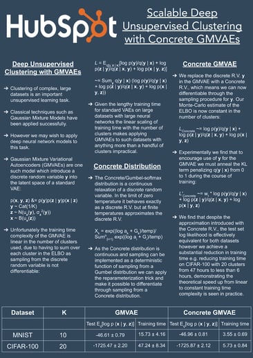It turns out that other researchers have developed deep neural network techniques that perform clustering. One such method is the Gaussian Mixture VAE (GMVAE). The GMVAE takes inspiration from GMMs in introducing a discrete random variable into the latent space of a Variational Autoencoder (VAE). VAE is a popular unsupervised learning algorithm. Clustering our dataset with off-the-shelf GMVAEs shows positive results. 

The problem with GMVAEs is that their training time computational complexity is linear in the number of clusters used. This means that if, for example, we expect our data to break down naturally into 200 groups, the time it takes to train the GMVAE will be approximately 100 times more than a dataset with 2 clusters. Thus when we apply GMVAEs to large, complex datasets with many natural clusters, the training can just take too long.

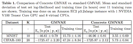
In our paper, we propose a solution to this problem by introducing a continuous approximation to the discrete latent variable in the GMVAE. This continuous approximation means the Monte-Carlo estimate of the GMVAE loss function has a complexity constant in the number of clusters. Experimentally, we find that this reduction in computational complexity corresponds to a remarkable decrease in training time under a realistic training setting. For example on CIFAR-100 (an image dataset) where we use 20 clusters, training time drops from 47 hours to less than 6 hours. Remarkably, we find that our approximation does not reduce the quality of the learned solution!

For the rest of this post, we will provide some of the more technical details of our method.

GMVAE

As with a VAE, for a GMVAE we imagine a process under which our data x was generated. Unlike a VAE, though, the generative process for a GMVAE involves a discrete variable y (think cluster ID). We imagine that each data point we see is the result of first randomly picking which cluster y the data point belongs to. Then we randomly choose some attributes z of the data point within the cluster. Finally, given these attributes, we produce the data point.

For example, consider a dataset of images of handwritten digits from 0-9. Under our generative process, we imagine that the images we see are the result of first thinking about which digit to draw, e.g. a number 2, then choosing what type of 2 to draw, e.g. a slanty one with a loop at the bottom, and then actually writing the number 2 on paper. This generative process can be described probabilistically:

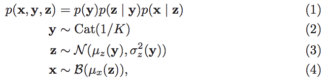
where y is described by a categorical distribution, z by a normal one, and x is Bernoulli distributed. Here each step in the process is parameterized by a (potentially deep) neural network.

Having defined our generative process, we need a way to train our neural networks. Ideally we would like to maximize the probability of our observed data, i.e. make the data we see as likely as possible. However, computing log p(x) (the logarithm of the probability of our data) is intractable. We instead settle for maximizing the Evidence Lower Bound (ELBO), an unbiased estimate of a lower bound on log p(x):

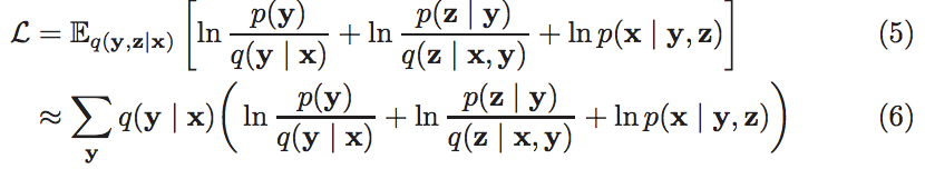
However, note that this estimate involves summing over all possible settings of the cluster id random variable y. This summation causes the training time complexity to be linear in the number of clusters used, which is the problem with GMVAEs that we seek to solve in our paper.

But why is this summation necessary? We note that in equation 6 we are approximating the expectation in equation 5. In making the approximation, we have sampled z ~ q(z | x, y). This gets rid of a high dimensional integral over z. The reason why we can’t do the same for y and sample y ~ q(y | x), is because y is discrete, so we cannot make the sampling procedure for y differentiable, which in the continuous z case can be done by the reparameterization trick. To train our neural networks we need differentiability.

Concrete GMVAE

Fortunately for us, there exists a continuous probability distribution designed specifically to approximate discrete random variables such as y. The Concrete distribution has the property that in the limit of zero temperature (a hyperparameter used to control the randomness of the sampling process) it becomes exactly discrete, but for non-zero, low temperatures is approximately discrete. We can apply the reparameterization trick to a Concrete distribution. This means we can sample from a Concrete distribution and differentiate through the sampling procedure.

In our paper, during training, we simply replace the discrete y with its Concrete approximation. As we can now sample y ~ q(y | x) and still get gradients for the parameters governing q(y | x), our unbiased estimate of the loss function becomes:

Notice how the loss now does not depend on the number of clusters. In practice, we find that using this estimate drives the Kullback–Leibler (KL) divergence between q(y | x) and p(y) to zero, causing the system to not do any clustering at all. This can be easily fixed by encouraging the system to use y by annealing the penalty on KL(q(y | x) || p(y)) from zero to one during training via a weight wt:

We test our Concrete GMVAE by comparing both training time and the quality of the learned solution on two image datasets; MNIST and CIFAR-100. We demonstrate that this theoretical reduction in training time complexity, is, in fact, borne out, when using a realistic training setup (i.e. one that includes early stopping, etc). The theory's predicted reduction in training time complexity from linear to constant scaling in the number of clusters (K) is observed.  Despite significant speedup in training time, our introduction of a continuous relaxation of the latent variable y in a GMVAE has had no significant negative impact on test set log-likelihood.

Thus where previously long training times made it practically impossible to apply deep learning powered GMVAEs to unsupervised clustering problems, our Concrete GMVAE makes it possible.. We hope that the Concrete GMVAE will prove useful for marketing, sales, and customer service professionals, as well as other users of clustering algorithms. and We also hope that our research will demonstrate the power of using continuous approximations to reduce the computational complexity of existing methods which sum over discrete random variables.